Notes on Viscous Term in Navier-Stokes' Equation

Image from Nottingham Math Department.

Navier Stokes Equation and Viscous Tensor

"TL;DR: A hand-wavy treatment of viscous term in N-S Equation. Refer to my future notes for a more rigorous one."

Let's consider the famous Navier Stokes' Equation:

\frac{D (\rho \vec{\pmb{v}})}{D t} = -\vec{\nabla} \cdot \overrightarrow{\bf{\mathrm{P}}}+ (\vec{\nabla}\cdot \pmb{\tau})^\mathrm{T} +\rho \vec{\pmb{f}}_{\mathrm{other}}

where $\frac{D}{Dt}$ is the total time derivative, $\rho$ is the density of fluid, $\vec{P}$ is the pressure, and $\vec{f}$ is some other forces on the fluid. $\cdot$ denotes inner product.

Here, for Cartesian coordinate $(x,y,z) \in \mathbb{R}^3$ ,

\pmb{\tau} = \begin{bmatrix} \tau_{xx} & \tau_{xy} & \tau_{xz}\\ \tau_{yx} & \tau_{yy} & \tau_{yz}\\ \tau_{zx} & \tau_{zy} & \tau_{zz} \end{bmatrix}

is a viscous tensor of rank two.

The reason we use a tensor to express forces is due to the fact each face of a fluid parcel suffers forces from left/right (along x-axis), front/back (along y-axis), and up/down (along z-axis). THIS IS AN IMPORTANT FACT.

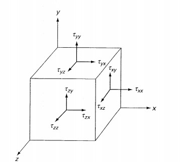
The first letter in the subscript of $\pmb{\tau}$ denotes the normal direction of the face, while the later one denotes the direction the force is pointing. This is demonstrated in the following diagram.

— Figure 1. Free body diagram of an infinitesimal fluid parcel. Image from Viscous Fluid by Frank White.

Viscous Tensor as Forces per Unit Area

To see that $(\vec{\nabla}\cdot \pmb{\tau})^\mathrm{T}$ gives us the correct description of viscous forces per unit volume $\overrightarrow{\mathrm{\bf{f}}}_{\mathrm{viscous}}$ on the fluid parcel, we consider, without loss of generality, the component of this force in the x direction.

It is not hard to see from Fig. 1 that the force in the x direction on the rightmost face is just the sum of each $\tau_{ix}$ that points to the right multiplied by the area of that face:

\mathrm{F_x^{right}} = \tau_{xx}(x+dx)\, dy\, dz + \tau_{yx}(y+dy)\, dx\, dz + \tau_{zx}(z+dz)\, dy\, dx

Hence, we can get the net viscous force by subtracting forces on the leftmost faces and the rightmost as

\begin{aligned} \mathrm{F_x^{net}} &= \mathrm{F_x^{right}} - \mathrm{F_x^{left}} \\ &= \frac{d \tau_{xx}(x)}{dx} dx\, dy\, dz + \frac{d\tau_{yx}(y)}{dy} dy\, dx\, dz + \frac{d \tau_{zx}(z)}{dz} dz\, dy\, dx \end{aligned}

Hence we have the x-component viscous force per unit volume $\mathrm{V_{par}}$ on the fluid parcel as

\begin{aligned} f_x &= \frac{\mathrm{F_x^{net}}}{\mathrm{V_{par}}} \\ &= \frac{d \tau_{xx}}{dx} + \frac{d\tau_{yx}}{dy} + \frac{d \tau_{zx}}{dz} \end{aligned}

Similarly, we have force per unit density $\bf{\vec{f}}$ as

\begin{aligned} \bf{\vec{f}} &= \begin{bmatrix} f_x \\ f_y \\ f_z \end{bmatrix} \\ &= \begin{bmatrix} \frac{d \tau_{xx}}{dx} + \frac{d\tau_{yx}}{dy} + \frac{d \tau_{zx}}{dz} \\ \frac{d \tau_{xy}}{dx} + \frac{d\tau_{yy}}{dy} + \frac{d \tau_{zy}}{dz} \\ \frac{d \tau_{xz}}{dx} + \frac{d\tau_{yz}}{dy} + \frac{d \tau_{zz}}{dz} \end{bmatrix} \\ &= \Biggr( \begin{bmatrix} \frac{d}{dx} & \frac{d}{dy} & \frac{d}{dz} \end{bmatrix} \begin{bmatrix} \tau_{xx} & \tau_{xy} & \tau_{xz} \\ \tau_{yx} & \tau_{yy} & \tau_{yz} \\ \tau_{zx} & \tau_{zy} & \tau_{zz} \end{bmatrix} \Biggr)^\mathrm{T} \\ &= (\vec{\nabla}^\mathrm{T} \pmb{\tau})^\mathrm{T} = (\vec{\nabla} \cdot \pmb{\tau})^\mathrm{T} \end{aligned}

Great! I think at this point it is clear why we use a tensor to express the viscous force.

Viscous Tensor is Symmetric

The reasoning behind this is that we don't want the fluid parcel to rotate. This is a physical assumption. If you think about water we drink being a giant cloud of rotating cubes, that would be really weird.

Expressing this fact in physical terms, we need the net angular momentum $\vec{\mathrm{T}}_\mathrm{par}$ of the fluid parcel to be $0$ .

We have by looking at Figure 1 again:

\begin{aligned} \vec{\mathrm{T}}_\mathrm{par} &= \begin{bmatrix} \mathrm{T}_x \\ \mathrm{T}_y \\ \mathrm{T}_z \end{bmatrix} \\ &= \begin{bmatrix} \tau_{zy} - \tau_{yz} \\ \tau_{xz} - \tau_{zx} \\ \tau_{xy} - \tau_{yx} \end{bmatrix} \\ &= 0 \end{aligned}

Hence, we proved that the tensor is symmetric since $\tau_{ij} = \tau_{ji}$ .

The Final N-S Equation

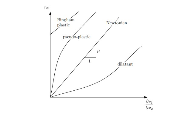
— Figure 2. A plot of stress versus speed change with height change in a fluid parcel determined by experiment.

Here we consider only Newtonian fluid ( $\mu$ is scalar constant). For some other fluid, where thermal effects come into play, you can refer to the full treatment given in the fluid mechanics notes by Dr. Joseph M. Powers at University of Notre Dame.

We see from Fig. 2 that we have the following equality:

\mu = \frac{\tau_{yx}}{\frac{\partial v_x}{\partial y}}

It is not hard to see that without loss of generality:

\mu = \frac{\tau_{ji}}{\frac{\partial v_i}{\partial x_j}}

assuming an isotropic fluid, i.e. $\mu$ is the same for each face.

In a more compact notation, we write the above as:

\begin{aligned} \mu \begin{bmatrix} \frac{\partial v_x}{\partial x} & \frac{\partial v_y}{\partial x} & \frac{\partial v_z}{\partial x} \\ \frac{\partial v_x}{\partial y} & \frac{\partial v_y}{\partial y} & \frac{\partial v_z}{\partial y} \\ \frac{\partial v_x}{\partial z} & \frac{\partial v_y}{\partial z} & \frac{\partial v_z}{\partial z} \end{bmatrix} &= \begin{bmatrix} \tau_{xx} & \tau_{xy} & \tau_{xz} \\ \tau_{yx} & \tau_{yy} & \tau_{yz} \\ \tau_{zx} & \tau_{zy} & \tau_{zz} \end{bmatrix} \\ \mu \vec{\nabla}(\vec{\pmb{v}}^\mathrm{T}) &= \pmb{\tau} \end{aligned}

Plugging this into the viscous force expression, we get:

\begin{aligned} \vec{\nabla} \cdot \pmb{\tau} &= \mu \vec{\nabla} \cdot (\vec{\nabla}(\vec{\pmb{v}}^\mathrm{T})) \\ &= \mu \begin{bmatrix} \partial_x & \partial_y & \partial_z \end{bmatrix} \begin{bmatrix} \frac{\partial v_x}{\partial x} & \frac{\partial v_y}{\partial x} & \frac{\partial v_z}{\partial x} \\ \frac{\partial v_x}{\partial y} & \frac{\partial v_y}{\partial y} & \frac{\partial v_z}{\partial y} \\ \frac{\partial v_x}{\partial z} & \frac{\partial v_y}{\partial z} & \frac{\partial v_z}{\partial z} \end{bmatrix} \\ &= \mu \nabla^2 \vec{\pmb{v}}^\mathrm{T} \end{aligned}

We hence obtained the usual Navier Stokes Equation:

\frac{D (\rho \vec{\pmb{v}})}{D t} = -\vec{\nabla} \cdot \overrightarrow{\bf{\mathrm{P}}} + \mu \nabla^2 \vec{\pmb{v}}^\mathrm{T} + \rho \vec{\pmb{f}}

and the transpose sign is just to get the row upright into a column, vector form.

References: (1) Viscous Fluid by Frank White. (2) Lecture Notes on Intermediate Fluid Mechanics by Joseph M. Powers, University of Notre Dame.